Benchmarking parallel programs is fraught with pitfalls. One often finds that understanding the performance of their program requires running multiple experiments with varying configurations and subsequently analyzing the data. One must deal with factors such as randomness in measurements, program faults, data collection and analysis. To cope with the complexity, one often writes a brand new, custom set of scripts, often in a scripting language such as python, perl or bash. It is all too easy for mistakes to creep into these scripts and for the errors to go undetected and lead to confusion or false conclusions. While this problem is inherent to any significant experimental study involving complex scripts, we believe that much can be done to reduce this problem in the particular case of studies which concern parallel codes on shared-memory machines.
In 2013, we began to develop a set of scripts, named pbench and written in the Caml programming language, that we could use to benchmark our parallel programs. Since then, we have generalized our scripts and have studied in detail a number of techniques to automate and ease the execution of experimental studies on parallel codes.
We have a few reasons to believe that others may find pbench useful. First, the scripts enjoy the correctness guarantees, such as type safety, that are enforced by Caml. Second, we have carefully designed a set of conventions and data structures for storing and processing experimental data. Third, we have designed the scripts to gracefully deal with program faults and timeouts. Fourth, we have implemented generators for several types of output formats, such as speedup plots, scatter and bar plots, and tables. We believe that, provided additional effort from others, these scripts can become a powerful tool to increase the rigor with which we analyze the performance of our parallel codes.
The software produced from these efforts consists of a pair of command-line tools, namely prun and pplot, and a library for writing custom experimental evaluations. The aim of the prun and pplot is to enable rapid experimentation with parallel codes in the early stages of an experimental study. In addition, we implemented a library to play the complementary role: that is, to provide a set of core functions that we could use to write Caml scripts to automate complex experimental evaluations of parallel codes. Our goal for these scripts is to make it as pain free as we could for us and others to repeat experiments that we report in our research papers.
In a related research effort, we have studied a lightweight performance-analysis technique for understanding the speedups obtained by given parallel codes (Umut A. Acar 2014). Although this study is still being prepared for publication, we post the draft here so that others may learn about our technique and provide us with feedback.
Our source code is hosted on a Github repository.
The manual page for the prun tool is available in PDF and HTML, for the pplot tool also in PDF and HTML.
We are going to present three small case studies and end with a link to a substantial case where we used pbench for the empirical evaluation in one of our research publications.
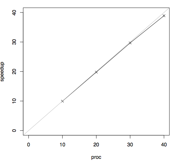
To get started, let us consider an experiment that is typical for parallel programming: one where the objective is to generate a speedup plot. For purposes of our demo, the speedup of a parallel program that is run on \(P\) processors in time \(T_p\) is defined by the ratio \(T_S / T_p\), where \(T_S\) denotes the running time of a corresponding sequential program. Our experiment is going to study a program which computes the forty-seventh Fibonacci number, using a naive exponential algorithm. This Fibonacci algorithm is the “hello world” algorithm of parallel programming.
In this experiment, for simplicity, we are going to use the same Fibonacci algorithm as both the sequential baseline and the parallel program. In general, however, the pbench speedup plot allows the sequential baseline program to be different from the parallel program. Now, suppose, for example that running time of the sequential baseline, which in our case is going to be the running time of the Fibonacci algorithm on a single processor, is \(T_S = 2s\). Further, suppose that the running time of the parallel program on 2 processors is \(T_2 = 1s\). Then, the speedup is \(T_S / T_2 = 2x\).
In this experiment, we have a binary, named fib, that takes as argument a number, -n 47, and a number of processors, -proc p, where we vary p. To run our experiment using ten processors, for example, we woud issue the following command and get something like the corresponding output.
$ fib -n 47 -proc 10
exectime 2.696
The output is printed by our Fibonacci program and, in this case, the output represents the running time in seconds that was taken to compute the forty-seventh Fibonacci number. In other words, this measurement was both taken internally and printed to stdout by our Fibonacci program.
Setting up the experiment with prun is not much more work. Our next step is to and collect data from one run of the baseline and four parallel runs, using ten, twenty, thirty, and forty processors. In order to get the corresponding command command lines from prun, we need the following formatting.
$ prun speedup -baseline "fib -proc 1" -parallel "fib -proc 10,20,30,
40" -n 47
The prun speedup part of the above command tells prun to perform a speedup experiment. Each speedup experiment requires three additional parts: the baseline-specific command, the parallel-specific command and the shared commands. In this case, our baseline command is fib -proc 1. This command is issued to prun by putting the command into the quotes after the argument -baseline. The parallel-specific command is specified in a similar fashion. All commands that are shared between the baseline and parallel runs must be specified once, after the -baseline and -parallel commands. In our example, the only shared command is the input size, which is specified by -n 47.
Note that fib, -proc 1, -proc 10,20,30,400, and -n 47 are specific to our fib program, whereas -baseline and -parallel are builtin keywords of the prun tool.
The command lines that are issued and the running times that are collected by prun are echoed to stdout. The data that is collected by prun is written by prun to the file results.txt.
[1/5]
fib -n 47 -proc 1
exectime 26.840
[2/5]
fib -n 47 -proc 10
exectime 2.696
[3/5]
fib -n 47 -proc 20
exectime 1.356
[4/5]
fib -n 47 -proc 30
exectime 0.904
[5/5]
fib -n 47 -proc 40
exectime 0.690
Benchmark successful.
Results written to results.txt.
Now, to generate the speedup curve, all we have to run is the pplot comand.
$ pplot speedupIf successful, the output is the following.
Starting to generate 1 charts.
Produced file plots.pdf.
The plot that we see should look like this one.
Our pplot depends on the R tool and LaTeX for generating plots. When pplot generates new plots, all intermediate R and latex sources that were generated by pplot are written to the _results folder. It is not hard to customize the look of the plots by editing these files individually.
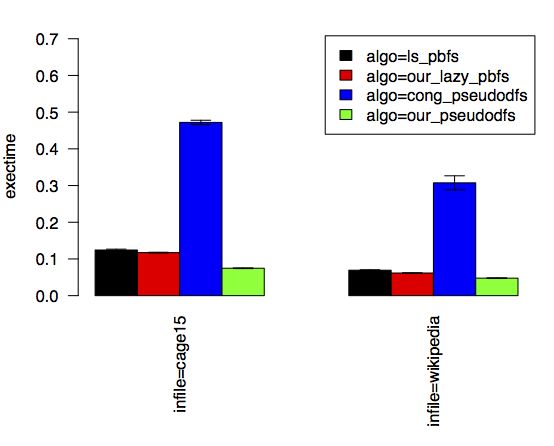
Now, let us consider how we might compare the running times of four different parallel graph-search algorithms using two different sample graphs. The following command line shows how we run one of these algorithms, namely ls_pbfs, using a few command-line arguments, such as -frontier ls_bag that are specific to this algorithm.
$ search -load from_file -infile cage15 -proc 40 -algo
ls_pbfs -frontier ls_bag -ls_pbfs_cutoff 512 -ls_pbfs_loop_cutoff 512
To get started, we are going to use prun to run the same command above and collect the data. Moreover, by specifying -runs 3, we are going to take three samples for this algorithm.
$ prun -runs 3 search -load from_file -infile cage15,wikipedia -proc 40 -algo
ls_pbfs -frontier ls_bag -ls_pbfs_cutoff 512 -ls_pbfs_loop_cutoff 512
After the run of the first three runs complete, we should have the data stored in results.txt. Now, let us perform the runs for the next algorithm, namely our_lazy_pbfs. Our use of prun is going to be the same, except for one additional argument: --append. This setting tells prun to append the newly collected data to the existing results.txt file.
$ prun -runs 3 --append search -load from_file -infile cage15,wikipedia -proc 40
-algo our_lazy_pbfs -our_lazy_pbfs_cutoff 128
We do the same for the algorithm cong_pseudodfs.
$ prun -runs 3 --append search -load from_file -infile cage15,wikipedia -proc 40
-algo cong_pseudodfs
And we do the same for our_pseudodfs.
$ prun -runs 3 --append search -load from_file -infile cage15,wikipedia -proc 40
-algo our_pseudodfs -our_pseudodfs_cutoff 1024
Finally, we can create a barplot from this data, we can simply issue the following command.
$ pplot bar -x infile -y exectime -series algo --xtitles-verticalThe plot that we get shows us bars grouped together by the input graph. On the y axis is the average of the three running times that we collected for each bar. We can see which algorithms are faster and, thanks to the error bars, how much noise there is in our measurements.
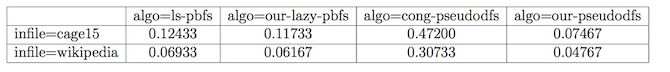
Using the same data as above, we can easily generate a table reporting on the running times.
$ pplot table -row infile -col algo -cell exectimeThe table that is generated is a latex table, and when rendered, looks like this one.
We used pbench to encode the experimental evaluation that was reported in our publication on a data structure called the chunked sequence. The sources for this evaluation are available from the chunked-sequence project page.
(Umut A. Acar 2014)
Get the bibtex file used to generate these references.
Umut A. Acar, Mike Rainey, Arthur Charguéraud. 2014. “Parallel Work Inflation, Memory Effects, and Their Empirical Analysis.” http://deepsea.inria.fr/pbench/work-inflation.pdf.